The MaxClueEntropy Strategy for WORDPL
In this blog post, I’ll describe how I won a delicious chocolate bar from Damien Desfontaines in his WORDPL contest with the MaxClueEntropy strategy. I’ll motivate why I picked this strategy, and I hope you’ll find my motivation at least a little bit pedagogically useful for explaining some basic concepts in information theory. Let’s start with a summary of the contest, so we’re all on the same page.
The contest
In case you somehow missed it, Wordle is a game in which you have to guess a secret five-letter word. After each guess, you get some feedback (a clue) that tells you which letters of your guess are compatible with the solution word and which aren’t. For example, if you guess ‘crate’ when the solution is ‘haste’, your clue will be \(⬛️\, ⬛️\, 🟨\, 🟩\, 🟩\).
WORDPL is a randomized variant of Wordle. In WORDPL, the clue is unreliable, because the color feedback for each letter is flipped with a certain probability. It is meant to illustrate the concept of differential privacy. Differential privacy is a formal privacy definition that provably limits how much information is revealed about any particular person in a data set. Differential privacy is quantified by a parameter \(\varepsilon\) — the lower, the stronger the privacy guarantee.
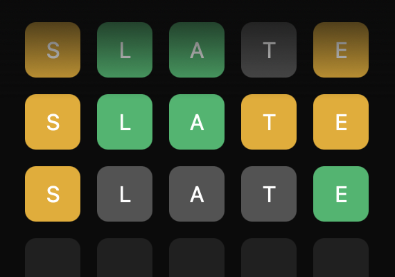
Due to randomness, you will get different clues even if you make the same guess multiple times:

A direct consequence of differential privacy is that it is impossible for any strategy to have a high chance of winning WORDPL for small values of \(\varepsilon\). But some strategies are worse than others, hence Damien Desfontaines called a WORDPL contest and promised chocolate to people who beat the high score. I entered with a strategy I called MaxClueEntropy.
The strategy
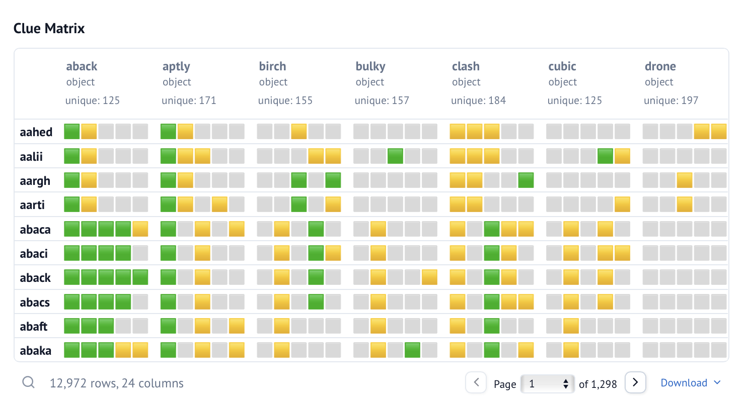
MaxClueEntropy is very simple: we guess the word for which we are the most uncertain about which clue we are going to get. We measure uncertainty by entropy, hence the name. To make this a bit more precise, let’s write \(\text{Clue}(g, s)\) for the true clue for guessing \(g\) when the solution is \(s\). For example, \(\text{Clue}(\text{cat},\, \text{tag}) = ⬛️\, 🟩\, 🟨\). It is helpful to arrange the clues for all possible (guess, solution) combinations in a table, which I call the clue matrix:

Click here for an interactive version of this table.
Of course, the actual solution is unknown to us, so let’s treat it as a random variable \(S\). At the first round, \(S\) is uniformly distributed over the solution list, because that’s how the solution word is selected. In subsequent rounds, it will follow the posterior distribution \(P(Solution \mid Previous\ Clues)\). In regular Wordle, \(P(Solution \mid Previous\ Clues)\) is uniformly distributed over the solution words that are compatible with all previous clues. In WORDPL, \(P(Solution \mid Previous\ Clues)\) is slightly more complicated, but Damien has described this well in his blog post, so I won’t go into it here.
On top of the randomness in the solution word, we also have the noise in the clues. Let \(\text{NoisyClue}(g, S)\) be the random variable describing the noisy clue we actually receive after making our guess \(g\).
Now, the strategy is to find the guess \(g\) that maximizes the entropy of the random variable \(\text{NoisyClue}(g, S)\), defined as \(\begin{align} H(\text{NoisyClue}(g, S)) = -\sum_{\hat{c}} P(\text{NoisyClue}(g, S) = \hat{c}) \log P(\text{NoisyClue}(g, S) = \hat{c}), \end{align}\)
where the sum is over all possible clues \(\hat{c}\). The noisy clue distribution can be computed as \(\begin{align*} P(\text{NoisyClue}(g, S) = \hat{c}) = \sum_{s} &P(Solution = s \mid Previous\ Clues) \\ &\cdot P(\text{NoisyClue}(g, s) = \hat{c} \mid Solution = s), \end{align*}\)
where the sum is over all possible solutions \(s\), and \(P(\text{NoisyClue}(g, s) = \hat{c} \mid Solution = s)\) is simply the noise distribution.
In other words, we go through each row of the clue matrix and count how frequently each clue occurs, weighted by our current belief of the solution word’s probability. Then, we pick the guess whose clue distribution has the highest entropy.
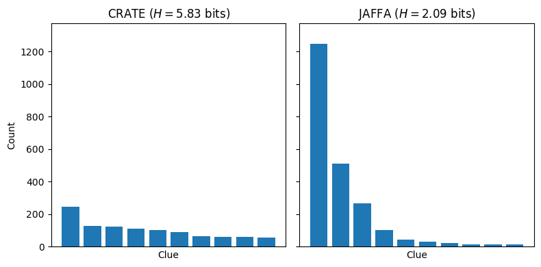
Here are some examples of clue distributions at the first round. The typical recommended starting guesses (slate, crate, etc.) have relatively uniform clue distributions.

Click here for an interactive version of the plot to explore the clue distributions of your favorite starting guesses.
Why clue entropy?
It is not immediately obvious why we should want our clue distribution to be as uniform as possible. What we really want is to reduce the uncertainty about the solution. So why not optimize for solution uncertainty directly?
My answer is that maximizing clue entropy is computationally convenient and actually equivalent to minimizing solution entropy. I’m offering two ways to show the equivalence: a quick and formal one, and an intuitive one. Let’s start with the formal one to get it out of the way. In information theory, there is an analogue to Bayes’ rule that looks like this:
\[\begin{align*} H(Solution \mid NoisyClue) = \ &H(Solution) - H(NoisyClue) \\ &+ H(NoisyClue \mid Solution). \end{align*}\]The terms \(H(Solution)\) and \(H(NoisyClue \mid Solution)\) are independent of our guess, therefore minimizing the left-hand side is equivalent to maximizing \(H(NoisyClue)\).
This was quick and painless, but not particularly insightful. For instance, you might still wonder: the entropy \(H(NoisyClue)\) is just a function of the clue probabilities and doesn’t care about the clue ‘values’. But some clues are clearly more informative than others. Surely, we would prefer, say, a 10% chance of observing \(🟩\ 🟩\ 🟩\ 🟩\ ⬛️\) over a 10% chance of observing \(⬛️\ 🟨\ ⬛️\ 🟨\ ⬛️\). Right?
Well, actually, no! And this is where I redeem my promise of a small bit of pedagogical value. A clue’s informativeness is truly, exactly, the same thing as its rarity. This is easiest to see in regular Wordle, so let’s ignore the noise for a moment and pretend \(NoisyClue = Clue\). Recall that, to compute a clue probability for a given guess, we walk through the corresponding row of the clue matrix and count how many times the clue occurs. If a clue occurs, say, 5 times, then we know that, if we were to observe this clue, we could narrow down the solution list to 5 words. That’s because any other solution word would have produced a different clue. Or, to state this more generally, if we observe a clue that has probability \(p\), this reduces the number of remaining solution words by a factor of \(p\). So we can actually see directly that the clue entropy is the expected order of magnitude by which the number of remaining solution words decreases:
\[\begin{align} H(Clue) &= -\sum_c P(Clue = c) \log P(Clue = c) \\ &= -\sum_c P(Clue = c) \log \frac{\left|\{\text{solutions compatible with}\ c\}\right|}{\left|\{\text{solutions}\}\right|} \\ &= -\mathbb{E}\left[\log \frac{\left|\{\text{solutions compatible with}\ Clue\}\right|}{\left|\{\text{solutions}\}\right|}\right]. \end{align}\]Results
In my simulations, the MaxClueEntropy strategy beats the NGuess strategy (the previous record holder) on the 50th and 95th percentiles, but not on the 5th. As far as I understand, NGuess simply plays a strategy that is known to be optimal for regular Wordle and disregards the clue noise. If you have an idea why the results might be so different for different \(\varepsilon\) values, please send me an email!
Optimizations
I will conclude with a few remarks on approximations I used in order to stay within the time limit in the contest.
- I restricted the search for guesses to the solution list. There are 12,972 allowed guesses and 2,315 possible solutions, so this a ca. 5.6x speed-up.
- Monte Carlo: I estimated the clue probabilities from only a small subset of columns that I selected via importance sampling, using \(P(Solution)\) as the proposal distribution. I sampled 200 out of the 2,315 possible solutions.
- I hardcoded the first guess, crate, which is optimal for \(\epsilon=0\).
It would be nice to explore ways to make this strategy even more efficient. For instance, can we exploit the fact that similar words have similar clue distributions to search the guess list more efficiently? I encourage you to try it out and submit a pull request!